Creating an Excel Drop-down List
Excel drop-down list can be based on:
a list of comma-separated values, a named range, and a range of cells
The methods described in this section apply to most of the Excel versions, including 2013, 2010, 2007 and 2003.
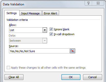
Creating an Excel drop-down list based on Comma Separated Values
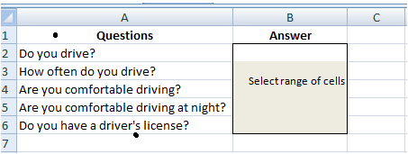
Select a cell or cells where you want the drop-down box to appear. It can be a single cell, a range of cells or the entire column as displayed in the illustration below. If you select the whole column, a drop-down menu will be created in each cell of that column. This turns out to be a time-saver for creating a questionnaire type of worksheet.
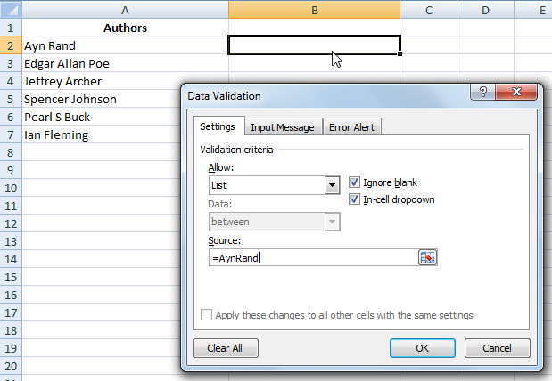
On the Excel menu bar click Data > Data Tools group and then click Data Validation.
The above method is feasible if you have only few cells residing on the Worksheet. If you want the same list to appear in multiple cells, then this method should be avoided. Editing will be cumbersome as you will have to change every cell that references the Data Validation list. Locating each cell and editing it can be a painful process. Here is a better way to do this.
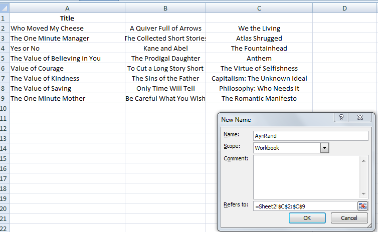
Creating an Excel drop-down list based on a named range
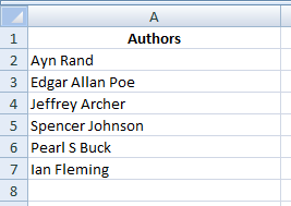
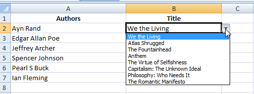
This method, though a bit time consuming, but it saves time in the long run. For example, let’s create a drop-down list of book titles of your favorite authors.
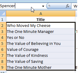
Alternatively, you can select the cells and type the range name directly in the Name box as illustrated below. When finished, click Enter to save the newly created named range.
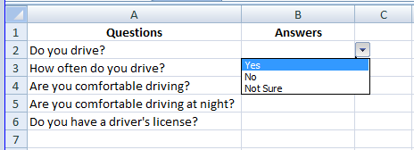
You can create book drop-down list for each author. A drop-down list with more than eight items will have a scroll bar. Note: You can create the list of items on the same or a different worksheet. For ease of understanding the example above uses two different worksheets.
Creating an Excel drop-down list based on a range of cells
This method is very similar to creating a drop-down list based on a named range except for a minor difference. When configuring your drop-down list, instead of typing the range’s name, click on the range selection icon next to the Source box, and select all cells with the entries you want to include in your drop-down list. They may be in the same or in a different Worksheet. If the latter, you simply go to the other Worksheet and select a range using your mouse. Designing a drop-down list in Excel is fairly easy and saves time. It is a clean method of displaying a large list of choices since only one choice is displayed initially until the user activates the drop-down box. We hope that this article on creating drop-down list in Excel was useful for you. Should you have any question on this topic, please feel free to ask in the comments section. We at TechWelkin and our reader community will try to assist you. Thank you for using TechWelkin!